A simple optimal control example

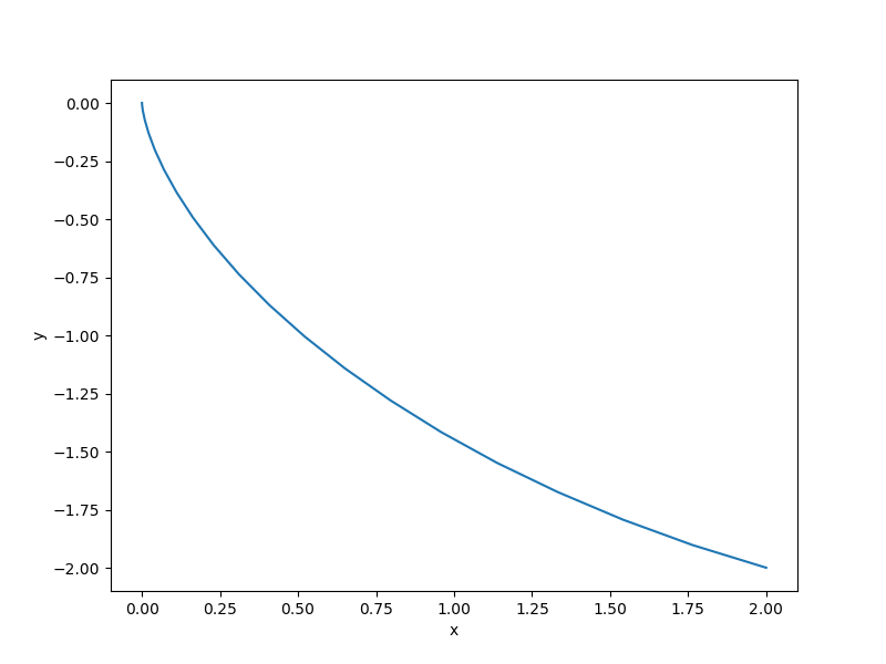
We illustrate how to use ozone to solve an optimal control problem - the Brachistochrone problem. We seek to find the curve along which a ball rolls from one point to another in the shortest amount of time. We minimize the final time, \(t_f\), by varying the dynamic control, \(\theta\), subject to the dynamics,

\[\begin{split}\frac{\partial x}{\partial t} &= v \sin(\theta) \\ \frac{\partial y}{\partial t} &= v \cos(\theta) \\ \frac{\partial v}{\partial t} &= g \cos(\theta). \\\end{split}\]

The initial conditions are

\[\begin{split}x(0) &= 0 \\ y(0) &= 0 \\ v(0) &= 0, \\\end{split}\]

and the transversality constraints are

\[\begin{split}x(t_f) &= 2.0 \\ y(t_f) &= -2.0 \\\end{split}\]

Here, we use the 6th order Gauss–Legendre collocation method with 20 time steps.

1. Defining the system

Here, our ODE function is defined by a single OpenMDAO system, an ExplicitComponent.

import numpy as np

from openmdao.api import ExplicitComponent


class GettingStartedOCSystem(ExplicitComponent):

    def initialize(self):
        # We declare a parameter for the class called num,
        # which is necessary to vectorize our ODE function.
        # All states, state rates, and dynamic parameters
        # must be of shape[num,...].
        self.metadata.declare('num_nodes', default=1, type_=int)

        # We make the acceleration due to gravity a parameter for illustration.
        self.metadata.declare('g', default=1., type_=(int, float))

    def setup(self):
        num = self.metadata['num_nodes']
        g = self.metadata['g']

        # Our dynamics depend on theta, x, y, and v.
        # They are all of scalars, so the overall shape is (num, 1).
        self.add_input('theta', shape=(num, 1))
        self.add_input('x', shape=(num, 1))
        self.add_input('y', shape=(num, 1))
        self.add_input('v', shape=(num, 1))

        # Our state variables are x, y, v, so we define rates for each.
        self.add_output('dx_dt', shape=(num, 1))
        self.add_output('dy_dt', shape=(num, 1))
        self.add_output('dv_dt', shape=(num, 1))

        # OpenMDAO assumes all outputs depend on inputs by default, so we first turn them off.
        self.declare_partials('*', '*', dependent=False)

        # dx_dt, dy_dt, and dv_dt are nonlinear in v and theta, so we only define
        # the sparsity structures of the Jacobians and not their non-zero values.
        self.declare_partials('dx_dt', 'v', rows=np.arange(num), cols=np.arange(num))
        self.declare_partials('dy_dt', 'v', rows=np.arange(num), cols=np.arange(num))
        self.declare_partials('dx_dt', 'theta', rows=np.arange(num), cols=np.arange(num))
        self.declare_partials('dy_dt', 'theta', rows=np.arange(num), cols=np.arange(num))
        self.declare_partials('dv_dt', 'theta', rows=np.arange(num), cols=np.arange(num))

    def compute(self, inputs, outputs):
        g = self.metadata['g']

        # This component computes dy_dt = -y.
        outputs['dx_dt'] = inputs['v'] * np.sin(inputs['theta'])
        outputs['dy_dt'] = inputs['v'] * np.cos(inputs['theta'])
        outputs['dv_dt'] = g * np.cos(inputs['theta'])

    def compute_partials(self, inputs, partials):
        g = self.metadata['g']

        theta = inputs['theta'][:, 0]
        v = inputs['v'][:, 0]

        # Earlier, we provided the structures of Jacobians; now we specify their values.
        partials['dx_dt', 'v'] = np.sin(theta)
        partials['dy_dt', 'v'] = np.cos(theta)
        partials['dx_dt', 'theta'] =  v * np.cos(theta)
        partials['dy_dt', 'theta'] = -v * np.sin(theta)
        partials['dv_dt', 'theta'] = -g * np.sin(theta)

2. Defining the ODE function class

Here, we define the ODEFunction, where we declare the 3 states and the control variable, which is called a parameter in ODEFunction.

from ozone.api import ODEFunction
from ozone.tests.ode_function_library.getting_started_oc_sys import GettingStartedOCSystem


class GettingStartedOCFunction(ODEFunction):

    def initialize(self, system_init_kwargs=None):
        self.set_system(GettingStartedOCSystem, system_init_kwargs)

        # We have 3 states: x, y, v
        self.declare_state('x', 'dx_dt', shape=1, targets=['x'])
        self.declare_state('y', 'dy_dt', shape=1, targets=['y'])
        self.declare_state('v', 'dv_dt', shape=1, targets=['v'])

        # We declare theta as a dynamic parameter as we will declare it as a control later.
        self.declare_parameter('theta', 'theta', shape=1)

3. Building the integration model and running

Here, we pass call ODEIntegrator to build our integration model and run it. The run script and resulting plot are shown below.

import numpy as np
import matplotlib.pyplot as plt

from openmdao.api import Problem, ScipyOptimizer, IndepVarComp, ExecComp

from ozone.api import ODEIntegrator
from ozone.tests.ode_function_library.getting_started_oc_func \
    import GettingStartedOCFunction

num = 21

# Instantiate our ODE function; use the solver-based formulation;
# 6th order Gauss--Legendre method; 20 time steps.
# We only provide the initial time and a normalized times vector
# since the final time is variable in this problem.
ode_function = GettingStartedOCFunction(system_init_kwargs={'g': -9.81})
formulation = 'solver-based'
method_name = 'GaussLegendre6'
initial_time = 0.
normalized_times = np.linspace(0., 1, num)
initial_conditions={'x': 0., 'y': 0., 'v': 0.}

# Pass these arguments to ODEIntegrator to get an OpenMDAO group called integrator.
integrator = ODEIntegrator(ode_function, formulation, method_name,
    initial_time=initial_time, normalized_times=normalized_times,
    initial_conditions=initial_conditions)

prob = Problem()

# Define independent variable components for final time and theta.
# Final time and theta are, simultaneously, component outputs and model inputs.
# We add our integrator group and components for our transversality conditions.
prob.model.add_subsystem('final_time_comp', IndepVarComp('final_time', val=1.0))
prob.model.add_subsystem('theta_comp', IndepVarComp('theta', shape=(num, 1)))
prob.model.add_subsystem('integrator_group', integrator)
prob.model.add_subsystem('x_constraint_comp', ExecComp('x_con = x - 2.'))
prob.model.add_subsystem('y_constraint_comp', ExecComp('y_con = y + 2.'))

# We issue connections using 'connect(output_name, input_name)'.
# src_indices is used when we just want to pull out a subset of entries in a larger array.
prob.model.connect('final_time_comp.final_time', 'integrator_group.final_time')
prob.model.connect('theta_comp.theta', 'integrator_group.dynamic_parameter:theta')
prob.model.connect('integrator_group.state:x', 'x_constraint_comp.x', src_indices=-1)
prob.model.connect('integrator_group.state:y', 'y_constraint_comp.y', src_indices=-1)

# We add the final time and theta as design variables, declare final time as the objective
# and add the transversality constraints.
prob.model.add_design_var('final_time_comp.final_time', lower=0.5)
prob.model.add_design_var('theta_comp.theta')
prob.model.add_objective('final_time_comp.final_time')
prob.model.add_constraint('x_constraint_comp.x_con', equals=0.)
prob.model.add_constraint('y_constraint_comp.y_con', equals=0.)

# We set the SLSQP optimizer as our driver in this problem.
prob.driver = ScipyOptimizer()
prob.driver.options['optimizer'] = 'SLSQP'
prob.driver.options['tol'] = 1e-6
prob.driver.options['disp'] = True

prob.setup(check=False)
prob.run_driver()

plt.plot(prob['integrator_group.state:x'][:, 0], prob['integrator_group.state:y'][:, 0])
plt.xlabel('x')
plt.ylabel('y')
plt.show()