A simple ODE example

We illustrate how to use ozone with the help of a simple example,

\[y' = -y , \qquad y(0) = 1 .\]

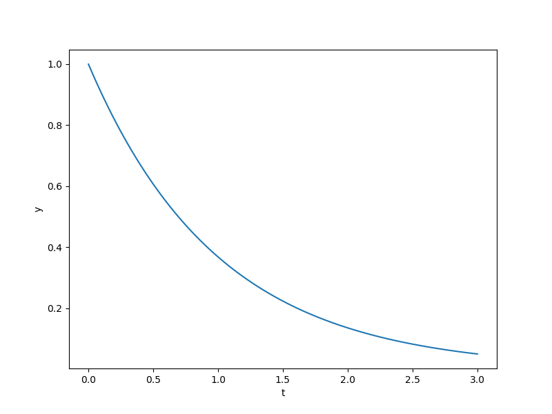
We integrate from \(t=0\) to \(t=3\) using 100 time steps of the 4th order Runge–Kutta (RK4) method. We use the solver-based formulation, which means the 100 time steps and the intermediate stages of the RK4 method are formulated as a nonlinear system of size ~400.

Building and solving an ODE in ozone consists of 3 steps.

1. Defining the system

Here, we define the OpenMDAO system that computes the \(\mathbf f(t, \mathbf y)\) function (in this case, \(-y\)). In this case, the system will be of type, ExplicitComponent, which is a unit of code that computes its outputs explicitly from its inputs.

import numpy as np

from openmdao.api import ExplicitComponent


class GettingStartedODESystem(ExplicitComponent):

    def initialize(self):
        # We declare a parameter for the class called num,
        # which is necessary to vectorize our ODE function.
        # All states, state rates, and dynamic parameters
        # must be of shape[num,...].
        self.metadata.declare('num_nodes', default=1, type_=int)

    def setup(self):
        num = self.metadata['num_nodes']

        # Our 'f' depends only on y, which is a scalar, so y's shape is (num, 1).
        self.add_input('y', shape=(num, 1))

        # dy_dt is the output of 'f'. dy_dt is also a scalar, so its shape is also (num, 1).
        self.add_output('dy_dt', shape=(num, 1))

        # The derivative of dy_dt with respect to y is constant, so we specify it here.
        # The Jacobian is diagonal, because each entry of dy_dt depends on the
        # corresponding entry of y, with a value of -1.
        self.declare_partials('dy_dt', 'y', val=-1., rows=np.arange(num), cols=np.arange(num))

    def compute(self, inputs, outputs):
        # This component computes dy_dt = -y.
        outputs['dy_dt'] = -inputs['y']

2. Defining the ODE function class

Here, we define the ODEFunction, where we declare the states, parameters, variable shapes, etc.

from ozone.api import ODEFunction
from ozone.tests.ode_function_library.getting_started_ode_sys import GettingStartedODESystem


class GettingStartedODEFunction(ODEFunction):

    def initialize(self):
        self.set_system(GettingStartedODESystem)

        # Here, we declare that we have one state variable called 'y', which has shape 1.
        # We also specify the name/path for the 'f' for 'y', which is 'dy_dt'
        # and the name/path for the input to 'f' for 'y', which is 'y'.
        self.declare_state('y', 'dy_dt', shape=1, targets=['y'])

3. Building the integration model and running

Here, we pass call ODEIntegrator to build our integration model and run it. The run script, resulting terminal output, and resulting plot are shown below.

import numpy as np
import matplotlib.pyplot as plt

from openmdao.api import Problem

from ozone.api import ODEIntegrator
from ozone.tests.ode_function_library.getting_started_ode_func \
    import GettingStartedODEFunction

# Instantiate our ODE function; use the solver-based formulation;
# 4th order Runge--Kutta method; 100 time steps from t=0 to t=3; and y0=1.
ode_function = GettingStartedODEFunction()
formulation = 'solver-based'
method_name = 'RK4'
times = np.linspace(0., 3, 101)
initial_conditions={'y': 1.}

# Pass these arguments to ODEIntegrator to get an OpenMDAO group called integrator.
integrator = ODEIntegrator(ode_function, formulation, method_name,
    times=times, initial_conditions=initial_conditions)

# Create an OpenMDAO problem instance where the model is just our integrator,
# then call setup, which is a mandatory step before running, then run the model.
prob = Problem(model=integrator)
prob.setup(check=False)
prob.run_model()

plt.plot(prob['times'], prob['state:y'][:, 0])
plt.xlabel('t')
plt.ylabel('y')
plt.show()

=================
integration_group
=================
NL: NLBGS 0 ; 52.915168 1
NL: NLBGS 1 ; 34.6412327 0.654656009
NL: NLBGS 2 ; 40.2500621 0.760652639
NL: NLBGS 3 ; 34.0182947 0.64288362
NL: NLBGS 4 ; 22.5016963 0.42524095
NL: NLBGS 5 ; 12.2126193 0.230796193
NL: NLBGS 6 ; 5.61726105 0.106155971
NL: NLBGS 7 ; 2.24129332 0.0423563489
NL: NLBGS 8 ; 0.789550019 0.0149210529
NL: NLBGS 9 ; 0.248964951 0.00470498273
NL: NLBGS 10 ; 0.0710497168 0.00134270984
NL: NLBGS 11 ; 0.0185172229 0.000349941683
NL: NLBGS 12 ; 0.00444070913 8.39212895e-05
NL: NLBGS 13 ; 0.000986197923 1.8637339e-05
NL: NLBGS 14 ; 0.000203933654 3.85397348e-06
NL: NLBGS 15 ; 3.94537699e-05 7.45604171e-07
NL: NLBGS 16 ; 7.17079955e-06 1.35515011e-07
NL: NLBGS 17 ; 1.22890677e-06 2.32240927e-08
NL: NLBGS 18 ; 1.99231818e-07 3.76511738e-09
NL: NLBGS 19 ; 3.06446142e-08 5.79127222e-10
NL: NLBGS 20 ; 4.48380089e-09 8.47356451e-11
NL: NLBGS 21 ; 6.25561197e-10 1.18219638e-11
NL: NLBGS 22 ; 8.34012991e-11 1.57613218e-12
NL: NLBGS 23 ; 1.0648684e-11 2.01240674e-13
NL: NLBGS Converged